Pong Game
The objective of the project is to defeat simple pong agent. We use different techniques and analyze them to find the optimal way to train our RL agent
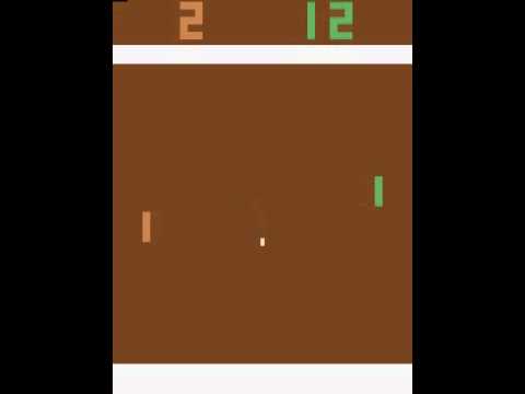
Pong is the most simplest of environments in atari games. We are provided with a variation of that environment build upon pygame. Despite being a simple game with only three actions UP, DOWN and STAY, the environment is difficult to learn for an agent. Our object is to try out different Reinforcement learning techniques and find out which works best for the agent. We started from vanilla Policy Gradient and analyzed its performance. We than tried A3C and its variants. The performance of agent with different techniques were then compared to see which one performed better
Background
Policy Gradient approach
We started with exploring the Policy Gradient (PG) algorithm as described by Andrej Karpathy. In its approach Policy Gradient as a general algorithm is used to train an ATARI Pong agent from raw pixels with a deep neural network. The reason PG is preferred over deep Q-network (DQN) is because it is end-to-end: there’s an explicit policy and a principled approach that directly optimizes the expected reward. Policy gradient methods have some major advantages over value based methods such as they can solve large and continuous action spaces without the need of discretisation (as in Q-learning). Moreover, value-based method cannot solve an environment where the optimal policy is stochastic. However Q-learning is beneficial in tabular cases and when you want deterministic policy. Mainly it also depends on the state representation of the problem as in some cases we would want to learn the value function and in others the policy. Figure below shows the flow of information in and out of neural network
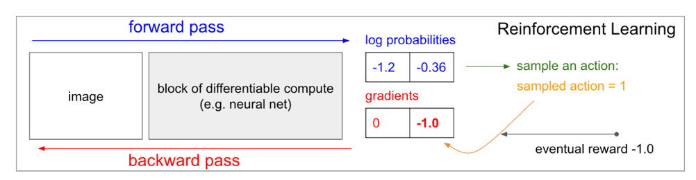
The approach mainly works by using a “policy network” which is 2-layer neural network with 200 hidden layer units. It is optimized using RMSProp on batches of 10 episodes that takes the raw image pixels (2101603) which are the difference of current and last frame. It produces log probability of the action which should be taken. After each action is executed (Up or Down) the game simulator gives a +1 reward if the ball went past the opponent, -1 if missed the ball and 0 otherwise. Conclusively, it learns a stochastic policy that samples actions which are either encouraged or discouraged based on the outcomes of the game.
Asynchronous Advantage Actor Critic (A3C)
Another external resource we reviewed is PyTorch implementation of Asynchronous Advantage Actor Critic (A3C) method. It is presented originally in a paper “Asynchronous Methods for Deep Reinforcement Learning” by Google’s DeepMind group. This variant of actor-critic approach maintains a policy and estimate of the value function uses asynchronous gradient descent for optimization of deep neural network controllers. The n-step methods operate in the forward view by using corrected n-step returns directly as targets.
This approach differs from DQN where a single agent represented by a single neural network interacts with a single environment. Whereas, A3C utilizes multiple incarnations of the environment in order to learn more efficiently. And since Actor-Critic combines the benefits of both value and policy based approaches, the agent uses the value estimate (the critic) to update the policy (the actor) more effectively than traditional policy gradient method. A3C also incorporates advantage estimates rather than just discounted returns. This allow the agent to determine not just how good its actions were, but how much better they turned out to be than expected.
It is shown in the study that this particular variant of actor-critic method performs better than Q-learning and SARSA approaches and also does so in half the time. Experimentation with the A3C approach also finds that using parallel actor-learners to update a shared model has a stabilizing effect on the learning process.
Implementation
Policy Gradient
We initially explored the policy gradient approach for our task. We followed a similar approach as described in the section above but since the resolution of input images is higher in our environment we standardize the pixels and instead of 200 hidden layer nodes we experimented with 200, 400 nodes and 500 nodes. We tried optimization with RMSProp and then with Adam. Also we experimented with initializing the weights randomly and then used Xavier initialization.
Out of these, the network with 400 nodes with Adam optimizer performed relatively better but it took a long time to train and it didn’t convergence.
Asynchronous Advantage Actor Critic (A3C)
The A3C implementation, as described in above section performs image processing to standardize the image and feed it to the network. The network architecture used to teach the agent remained the same. The observation image we get is different than the general Atari game observation. The environment image consist of 210 x 210 x 3. Before feeding the image into the network the image is sampled down to 80 x 80. This transformation is performed in two steps to avoid loss of pixels on the edge of frame. The image is first down sampled to 105 x 105 x 3 in the first step, in second step the image is further sampled down to 80 x 80 x 3. Furthermore, the image is converted into 1D image by taking average in all the dimensions. Once the image is in standard form the columns of the image are normalized to make them unbiased.
The processed image is fed into the neural network. As specified in A3C architecture the network is divided into two categories Convolutional layers to process spatial dependencies and LSTM layer to process temporal dependencies, the final output is then passed to 2 fully connected layers for actor and critic values. The neural network architecture is same as the universal architecture. The network consist of 4 CNN layers followed by 1 LSTM layer. The details of different layer specifications is shown in Table below. The weights of the neural network are initialized using Xavier initialization, which was selected because it tends to initialize the weights so that the result falls in the range of the activation function of layers, and is preferred generally when training deep neural nets.
| Layer Type | Specification |
|---|---|
| CNN | 32 x 32 kernel with 1 padding and stride of 2 |
| LSTM | 256 cells |
| Actor | 1 layer with 256 nodes, output equal to number of actions available |
| Critic | 1 layer with 256 nodes, output equal to number of actions available |
For each step the normalized observation/state is fed into the neural network. The actor output is fed into softmax layer and a single action with maximum probability is sampled out from multinomial distribution using the output of softmax unit. The log probability of the actor softmax is used to find the entropy of the policy which is used in citric loss function.
Each worker plays game for 20 iterations. At the end of each iteration the worker uses the entropy and the values of policy and critic to update the network. Generalized Advantage Estimation (GAE) is used to update the values of policies for the network. This method is selected as it gives low variance compared to conventional advantage functions. The hyper parameter for the GAE were not changed. Tau is set to 1.00, gamma to 0.99, energy coefficient of 0.01 and value loss coefficient of 50. The batch size of 20 iteration was selected after some experimentation, it was observed that 10 iterations were too low to learn anything initially as the agent was naive and the game did not lasted longer than 22 steps. When the steps were changed from 10 to 20 the agent was able to learn better actions.
The optimization algorithm was changed from conventional RMSProp to Adam. The choice of optimization algorithm is again due to the better performance of algorithm even in noisy conditions as compared to RMSProp
Reward Evaluation
To learn about the behavior of agent 2 kinds of reward functions were introduced in the environment. The first one was simple reward function which give reward of +10 when the agent wins the game and reward of -10 when the agent losses the game. The second reward function set the reward to -10 in either case of win or loss of game for the purposes of extending the episode length so that the agent plays defensively. The two reward functions were evaluated in the A3C environment described above.
Results and performance analysis
The configurations and the environment setup described above were evaluated on test setup of 20 games. It was observed that vanilla policy gradient agent was unable to learn well on the environment. It showed confused behaviour for all the configurations. The reason for this kind of behaviour could be lack of image pre-processing. Furthermore, it is also known that Deep Reinforcement Learning algorithm are very sensitive to hyper parameter tuning, it could be possible that the hyper parameters were not tuned properly for vanilla policy gradient to work.
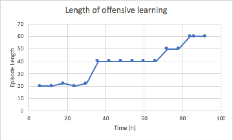
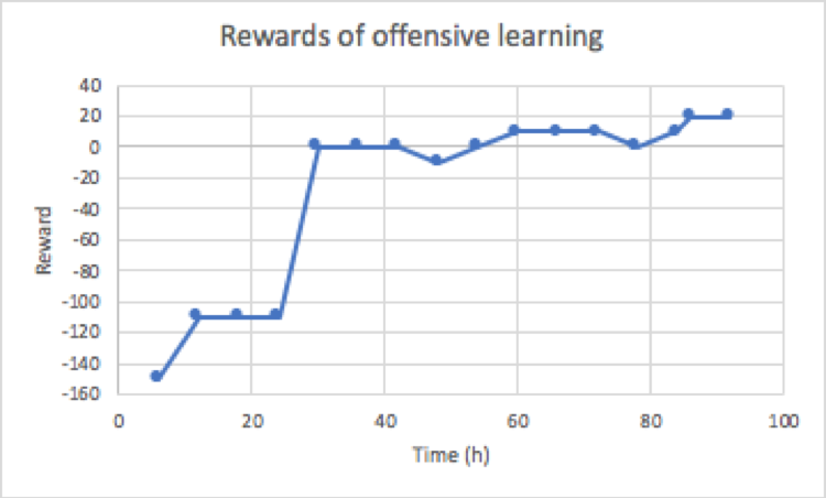
The agent learned on the above mentioned settings. The number of individual workers were set to 4. The agent learned on the above mentioned setting for 4 days. Two A3C agents were instantiated to differentiate and compare the performance of different reward functions mentioned above. The agent which gets +10 when it wins is calls offensive agent and the agent with -10 reward when it wins is called defensive agent. The graphs in Figures below shows the performance of offensive agent. The graph shows that the agent started as a naive agent and wins only some games by luck. However, after training for few hours it improved and started to win almost half of the games within 2 days. The progress after 2 days was as steady and in the coming 2 days it only improved from 50 to 70. If we look at the length of the game it shows steady increase which means that agent was able to anticipate the moves of the opponent and follow the ball even and hit it more than once per game, still it could be seen that the agent was unable to go beyond 3 hits after 2 days.
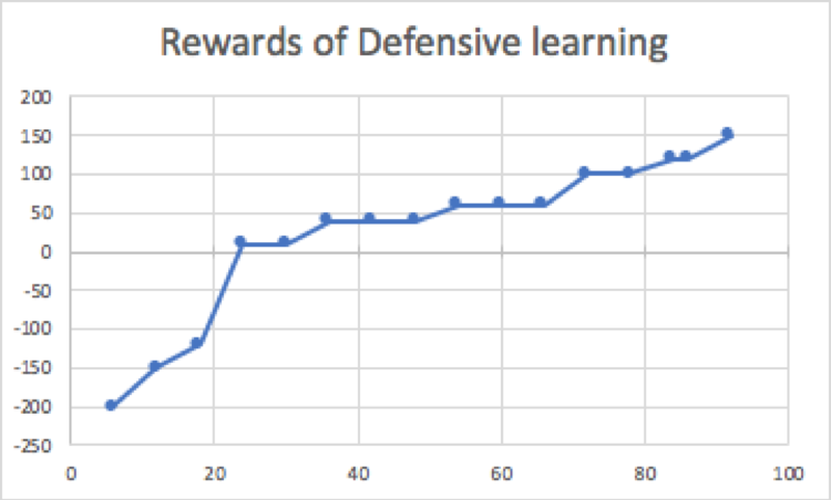
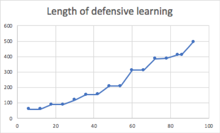
Contrary to the offensive agent, defensive agent started with a high negative reward. Figures below show the performance of defensive agent. This means that most of the time the agent was losing the game. However, the initial episode length was larger than that of offensive agent and it continues to grow as the time passed, showing that agent was learning to make longer games than to win. The surprising observation was that the agent was able to beat the opponent in the process. The reason for this behavior could be simple ball following approach of simple ai agent. Another explanation of this behavior could be that the agent overfitted on the simple ai agent and was able to counter most of the moves made by the agent. Comparing the two techniques show that defensive agent was able to learn fast in this environment with simple ai agent as the opponent than aggressive agent.
As the final experiment the two agents were competed with each other and it was observed that the offensive agent dominated the game. One reason for this behavior could be that the defensive agent was expecting the other agent to play defensive as well whereas offensive agent was trying to win the game. Another reason as mentioned above could be that the defensive agent has overfitted the simple ai agent.
Conclusions
Based on our experiments we can fairly conclude that the A3C approach resulted in better outcomes than traditional Policy Gradient method. We further found that using an actor critic approach for this task of making an agent to learn play Pong would is more effective as we have learned during the progress of the course that Actor-Critic methods offers the strengths of both value based and policy gradient methods.
Furthermore, A3C approach provides a novel way to make the agent learn faster and effectively better than other methods we explored. However, there is always room for improvement and the neural network architecture can be experimented with more. Also we can apply experience replay techniques to improve the learning time.
The code base for pong project could be found here