Email Marketing

This project uses Q Learning based Reinforcement Learning agent to predict optimal time for sending multiple category emails to different type of users

Introduction

For email campaign, the traditional problem is to personalize email to clients. The problem could be divided into several sub problems including but not limiting to finding most effective time period to send the email, personalize the content of the email depending on feature extracted from client. One way to approach this problem is to observe the patterns of interactions people have with emails and try to depict their behavior. A stream of interactions occurs between the company and each customer, including actions from the company (such as emails) and actions by the customer (such as registering to advertised campaign). Understanding user decisions is a problem gaining increased interest in today’s research. Mining behavior patterns has been used to discover users that share similar habits and using sequential patterns to learn models of human behavior has been employed in lifestyle assistants to increase the life quality of elderly people. Research has been done to automate different aspects of campaigning problem using Reinforcement Learning.

In this report we simulate the user behaviour to email campaigns and try to build a Reinforcement Learning agent that would optimize email campaigns by analysing category of email and time at which email was sent. The agent performs well on simulated data, it is able to find times when it is optimal to send email to users, it also categorize the users into campaigns that they respond to positively.

Reinforcement Learning

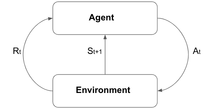
Reinforcement learning (RL) is a branch of machine learning which allows agents to interact with the environment by sequentially taking actions and observing rewards to maximize the cumulative reward. Figure below can be used to understand general flow of RL system. The agent takes action A_t which effects the environment. The environment than generates the next state S_t+1; which could depend upon action performed A_t and current state of the system S_t; and the reward R_t for the agent. The agent based on the feedback provided by the environment decides which action to perform next. This action feedback loop continues until certain condition is satisfied. Environments play an important role in RL systems, generally we generate simulations of actual environment to train the agent. Factors taken into account when simulating the environment decides how well the agent performs in real scenerios. Environments in RL domain are typically divided into two categories: episodic and continuing environments. In an episodic environment, the interaction sequence eventually terminates, at which point the environment resets and a new interaction sequence begins; whereas in continuing environments, there is a single interaction sequence that never terminates.

Fig 1: Basic Reinforcement Learning flow

RL problems can be modeled as Markov Decision Process (MDP), MDP is defined as a tuple (S, A, R, P). Where $\textbf{S}$ represents the state space. $\textbf{A}$ represents the action space, $\textbf{R}$ is the immediate reward, and $\textbf{P}$ is the state transition dynamics. For a certain process there exists a policy $\pi$ on $\textbf{A}$ . The agent moves through the state space according to the actions provided by the policy. The set (s $_{i}$ ,a $_{i}$ ,r $_{i}$ ), state, action and its reward that agent follows is known as trajectory of the agent. The equation below is used to represent optimal policy for RL systems.

$\begin{gather*} \pi^{*} = \text{arg max}_{\pi} E[\sum^{\infty}_{t=0}\gamma^{t}r_{t}| \pi] \end{gather*}$

Here $\gamma$ [0,1) is called the discount factor. The value of $\gamma$ determines the affect of future states on current state. If value of $\gamma$ is close to 0, the future states have little or no affect, whereas if the value is close to 1 future states have same affect as states close to the current state. The other term inside summation is , it represents the reward achieved by agent at time step t, by following policy $\pi$ . Summation over terms described above represents one of the trajectories followed by agent under policy $\pi$ . The goal of the RL algorithms is to learn an optimal policy $\pi^{*}$ which maximizes the expected return from the initial state.

In case of our email campaign problem, the emails are sent to different client, interactions with different kinds of marketing mails are the actions which changes the state of MDP. The sequence of actions performed by user creates a policy. We are provided with full policy or a part of policy. The environment for this problem is considered to be episodic.

Q Learning

Q-learning is a form of model-free reinforcement learning. Q-learning agents could learn to act optimally by experiencing the consequences of actions. Q-learning is one of the off policy algorithms, that means the learned Q function directly approximates $\pi^{*}$ , independent of the policy being followed. Learning proceeds similarly to method of temporal differences (TD): an agent tries an action at a particular state, and evaluates new value of state it is in. By trying all actions in all states repeatedly it learns approximation of $\pi^{*}$ . In order for agents to learn evaluation of action for a particular state is required, for this purpose state-action pairs Q(S $_{t}$ ,A $_{t}$ ) also known as Q values are used. If agent can only perform discrete and finite actions, and there are finite number of states, the state action pairs could be stored in a tabular form. In tabular form of Q learning agent updates Q values in each episode. After the convergence is achieved agent uses learned Q values to decide which action to perform. The equation below shows the update rule for Q-learning.

$\begin{gather*} Q(S_{t}, A_{t}) \leftarrow Q(S_{t}, A_{t}) + \alpha \big[ r_{t+1} + \gamma \text{max}_{a} Q(S_{t+1},a) - Q(S_{t}, A_{t}) \big] \end{gather*}$

The equation have two hyper-parameters that are to be set manually. First one is discount factor $\gamma$ which decides the contribution of next state Q value on updated Q value of current state. However, as shown in the equation next state Q value of the best action is selected. The second hyper-parameter is $\alpha$ , it determines how much the updated value contribute to Q value of current state, if value of $\alpha$ is small the learning is slow where as if the value of $\alpha$ is large agent could miss optimal Q value. The value of hyper-parameters are selected through trial and error methods like grid search and random search. Using the update definition defined above and assuming that all Q values continue to update, the algorithm converges to $\pi^{*}$

Method

The basic email campaign problem is divided into two part. The first part is to find the optimal time to send emails. Optimal time here is considered to be points in time when clients give positive feedback. Secondly, it is required to find the categories in which client belongs. This will reduce the number of emails sent to clients, only clients with positive feedback to specific category would be pursued.

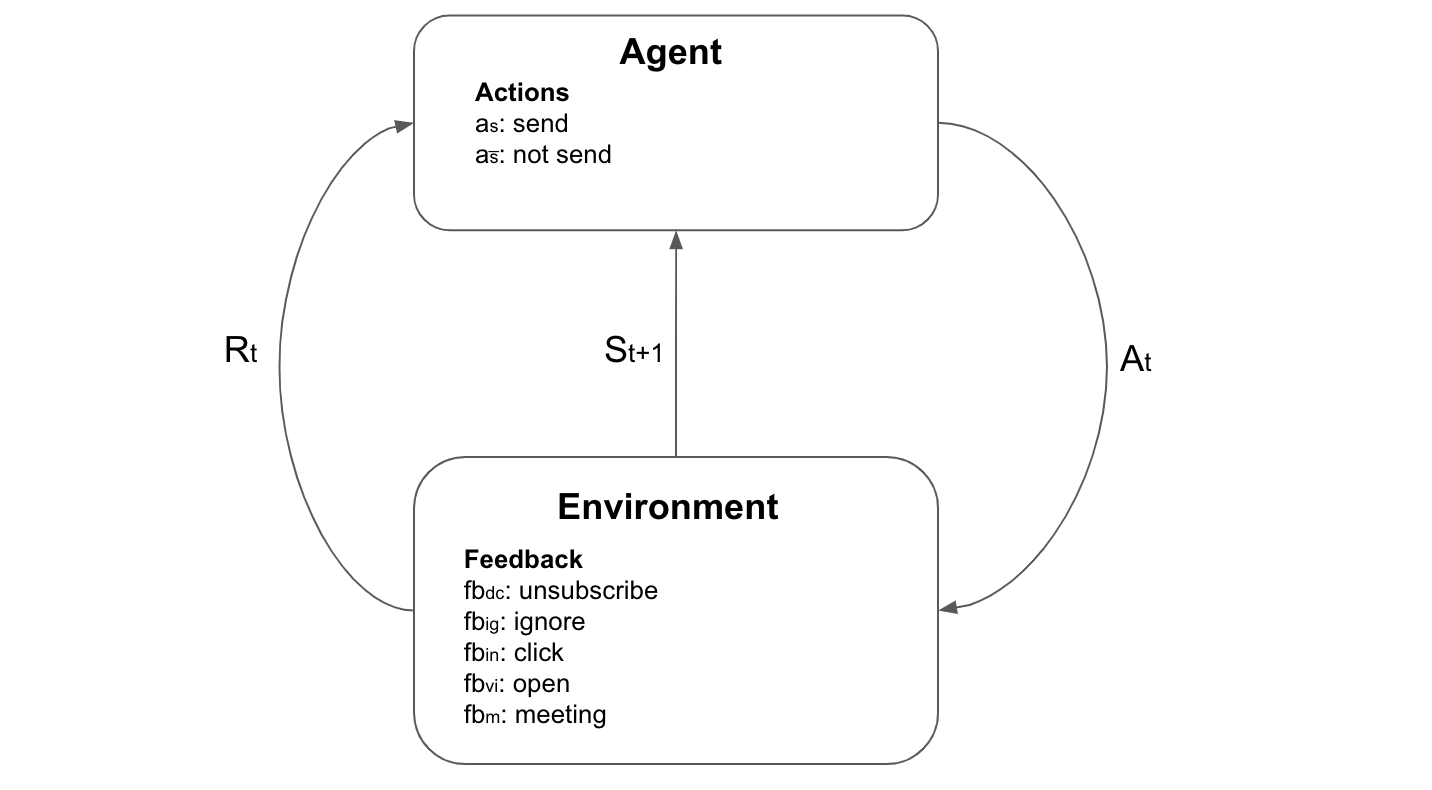
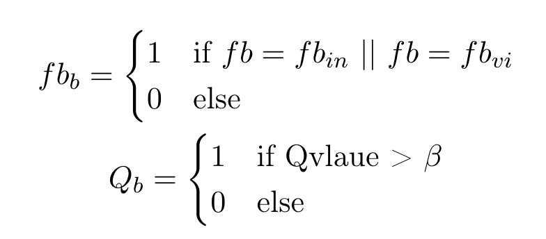
We start by defining action feedback model. The agent has two actions that it could perform. It could either send the mail to the $a_{s}$ , or it could remain idle $a_{\bar{s}}$ . The user in return could provide with one of four feedback. The user can either unsubscribe fb $_{\text{dc}}$ , ignore the mail fb $_{\text{ig}}$ , click on the mail sent fb $_{\text{in}}$ or open the advertisement link sent in the mail fb $_{\text{vi}}$ . The model described is shown in Figure below. The selection of rewards is discussed next section.

Fig 2: Flow of RL Agent for email marketing

Preference State Transitions

Fig 3: Preference State Transitions

Non Preference State Transitions

Fig 4: Non Preference State Transitions

User Simulation

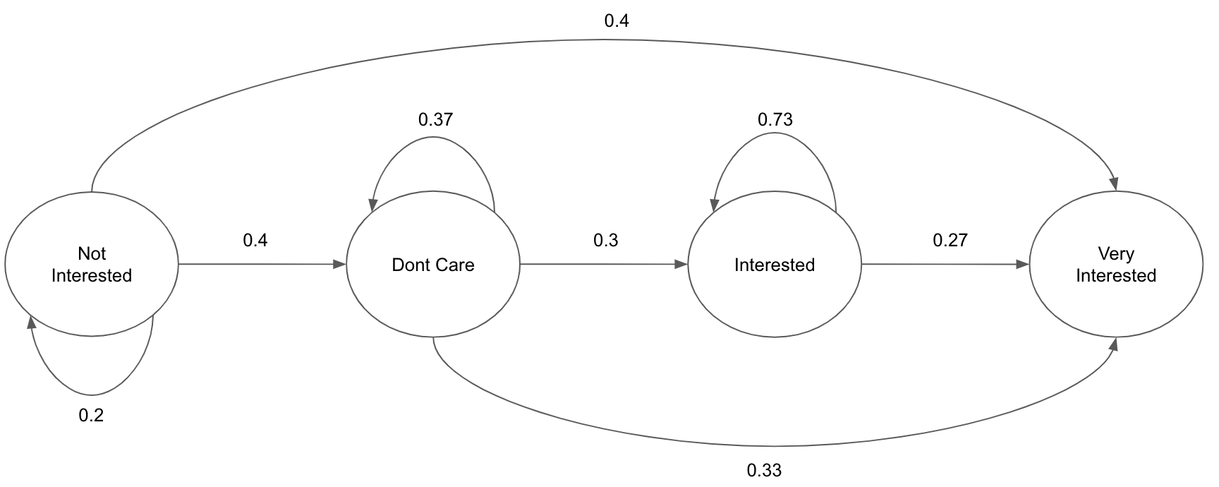
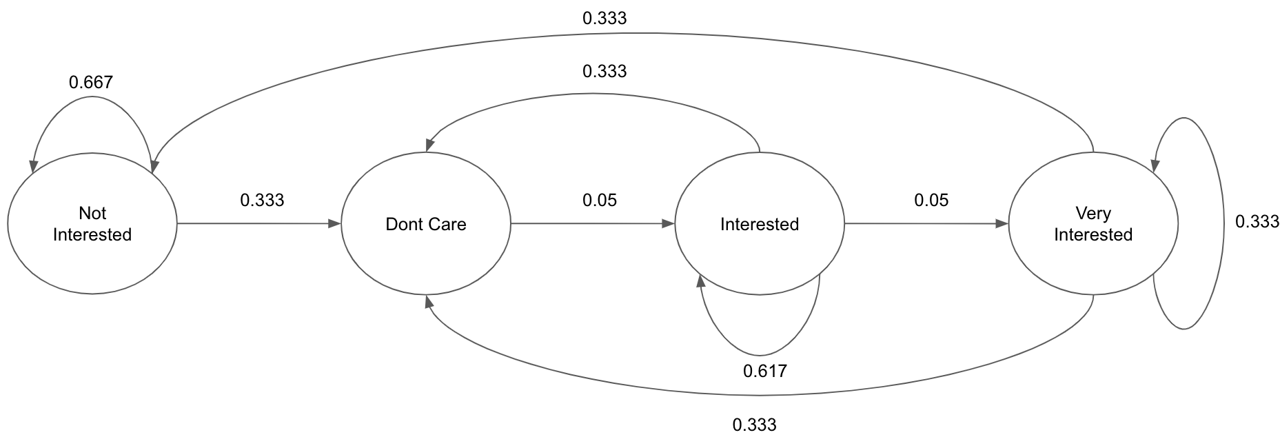
Once basic model for reinforcement learning is specified, next step is to simulate the environment. In this case user response was simulated. Before analysing the data, emails were divided into two categories; namely preferential and non preferential emails. Data was used to extract transition probabilities for user feedback. The report for data processing and feature extraction could be found here. Fig: 3 and Fig: 4 show prominent transition probabilities for both email categories. The initial state of every user was set to fb $_{ig}$ . The number of users, number of categories, number of preference categories per user and time steps are tunable parameters of simulated data. The prior of user response was generated using transition matrices. On the time of training a random variable $\eta$ was introduced which accounted for the randomness of user behaviour.

A binary variable $c$ was introduced that could take values from $C$ $\in$ { $p$ , $\bar{p}$ }; to user response simulation, where $p$ represents preference category and, $\bar{p}$ represents non preference category. The prior feedback is generated using the transition probabilities as described in Method section. Hence, the prior could be defined as follows:

$\begin{gather*} P(fb | C = c) = \text{Transition probabilities} \hspace{5mm} C \in \{p, \bar{p}\} \end{gather*}$

Agent

The objective of agent is to find optimized time and preferred categories for each user. The agent is specified by the tabular state space consisting of 365 time steps representing days in a year. Agent was further divided into several mailing lists agents represented by m $_{k}$ $k$ $\in$ [1, $\ldots$ , n]; representing the number of categories of mailing list present within an agent. Initially, emails of all categories are sent to every user. The agent is than expected to learn which email should be sent to which user. The initial state of system is shown in Fig 5.

Cat overview

Fig 5: Mailing list overview

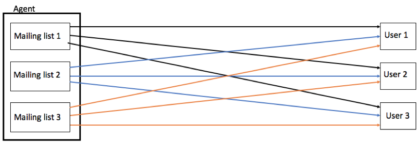
The space state for this system is different than conventional state space used in Q Learning. We train a separate model for each mailing list to find users who have high acceptance probability for that category. The action space of each agent in this scenario is equal to the number of users present in that mailing list. Hence, the tabular state space that agent needs to learn would consist of number of users x 365. Initially, agent will start with zero valued state space. As learning progresses, agent learns Q values for each user. Preferential users are expected to have more positive response than non preferential users, resulting in greater number of positive Q values.

Experiments and Results

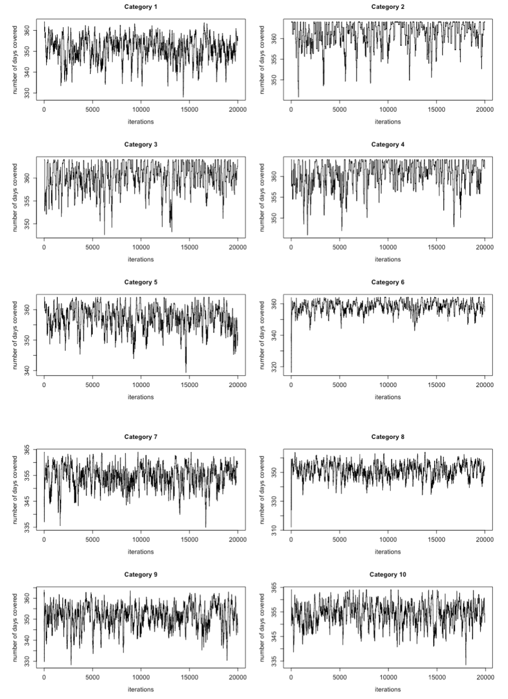
The system described above was configured to have 10 mailing lists and 5 users. Decaying exploration with $\alpha$ = 1000, was used to allow agents to explore the state space initially in training phase. The learning for system was performed for 20000 episodes; each with 365 time steps, Fig 6 shows of graph of iterations for all 10 mailing lists. There are two types of graphs that could be observed. First type of mailing lists were able to complete 365 time steps from the beginning of training, these mailing lists were the ones that were not selected by any user as preference category. One such example could be Category 1, which show steady trend throughout all episodes. Second type of mailing lists start with small number of time steps in beginning of training and gradually learn to converge near 365 time steps. These mailing list are part of one or many users preference category list. Category 2 is one of the mailing lists that initially had lot of noise in the training steps but after 15000 iterations become more stable.

Cat overview

Fig 6: Iterations

After the mailings lists were trained. We had Q values for every user for every mailing list. To correlate the response of user to the Q values we converted them both into binary variables. The equations below shows how the Q values and user feedback was converted into binary variables. As the equation below shows $fb_{b}$ is the binary representation of user feedback showing user interest. $Q_{b}$ is the binary representation of Qvalues learned by the agent, $Q_{b} = 1$ shows that agent should sent the mail at that time instance to the specified user, whereas $Q_{b} = 0$ means mail should not be sent. This conversion of Qvalues consist of $\beta$ which is hyperparameter and could change depending on the number of mailing lists and users in the system. The system defined above has value of $\beta$ set to 25.

eq-1

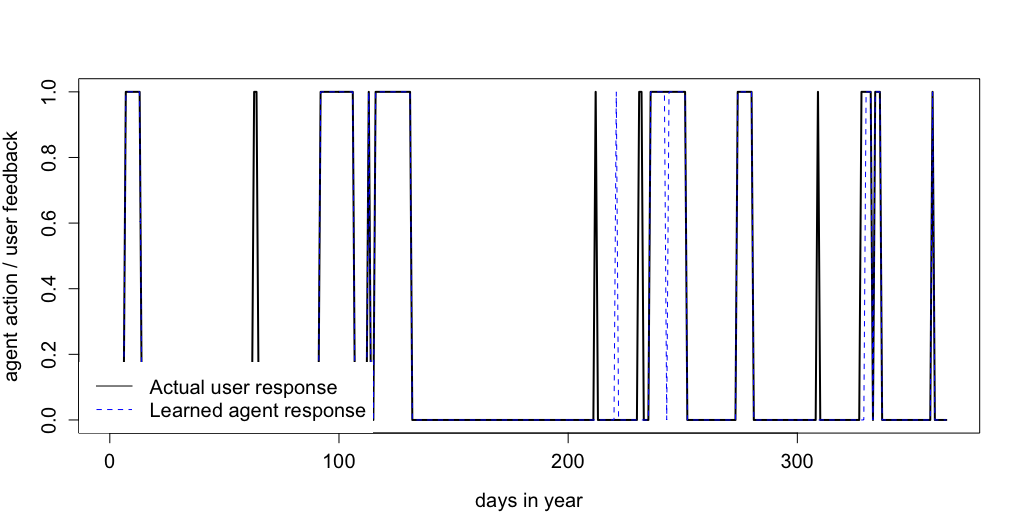
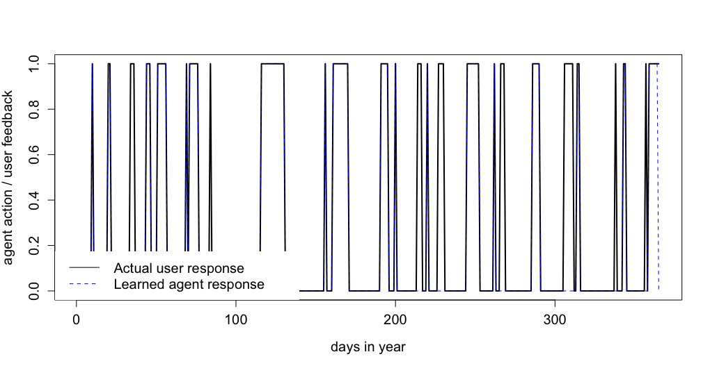
To test the training accuracy of the system a preference user and a non preference user was chosen at random Fig 7 and Fig 8 show the results respectively. The visual analysis show that there were less positive response from non preference user as compared to preference user. Furthermore, it shows that agent was able to learn when to send mails to both preference and non preference user. However, to analyze the learning process in more depth confusion matrices were created for preference and non preference user Table 1 and Table 2 shows the result respectively.

res-pref

Fig 7: Results of preference category user

res-non-pref

Fig 8: Results of non preference category user

	neg feedback	pos feedback
not sent	266	23
sent	0	76

Table 1: Confusion matric of Preference user

	neg feedback	pos feedback
not sent	287	9
sent	1	68

Table 2: Confusion matric of non Preference user

The confusion matrix confirms the findings of the graphs, for preference users agent was able to correctly classify 93% of time steps. There was no misclassification for negative feedback. However, agent was successfully able to cover 76% of user positive feedback. Total misclassification was about 6.3%. For non preference user agent was able to correctly classify 99% of user negative feedback and 88% of user positive feedback. The total misclassification for non preference user was 5.2%.

Overall, the experiments using the defined system suggests that agent is able to learn user patterns for different mailing list with high accuracy.

Conclusion

In this report we tried to solve the problem of email campaign using tabular Q Learning technique. We used real data to extract statistics which were than used to create user behavior simulations. The system of different mailing lists was trained on that simulation. The results show that system learned quite well when to send data to which user for a specified category. One limitation for the system is that it keeps the learned Qvalues in the memory, the memory requirement of system would increase when we add more categories and more users per category.

The code for this project could be found here